Recently at work, I started to reuse the ALS algorithm in the PySpark MLlib package to build user and item factors. This algorithm, quite famous in recommender systems, is based on the concept of matrix factorization (MF), which is familiar in the dimensionality reduction area of machine learning. I thought that discussing matrix factorization could make a good article since it’s a powerful technique.

This article will present the core concepts of matrix factorization, along with a non-exhaustive list of popular algorithms highlighting their specific features and cover a few key points to keep in mind when using matrix factorization for recommender systems.

Ratings at the core of the factorization

So, what is matrix factorization in the context of recommender systems? Typically, it involves taking a user-item ratings (often referred to as feedback in the literature) matrix and factorizing it into two matrices: one for users and one for items (Example).

Where do these ratings come from ?

• Explicit: A user gives a score to an item based on their preference and on a dedicated scale. One famous example is Amazon’s 5-star rating system.

• Implicit: A user interacts with the items in the catalog of your application, and based on these interactions, we can determine the user’s implicit preferences. For example, if you’re watching some TV shows on Amazon Prime, you might finish some and not others, or you might visit the content page for some items but not others. These interactions can reveal implicit preferences within the catalog.

Note that Prime Video also offers the ability to thumbs up or thumbs down the content in its catalog.

In both cases, ratings are defined on a specific scale (e.g., 0 to 5, 👎👍, or 0 to 1). They are built on top of user interactions with the catalog, and in any application, the company’s strategy can evolve over time. A good example of this is Netflix. I’ve compiled a few resources on Netflix’s changing strategy over time regarding the collection of user feedback. Here are some key milestones:

• In 2009: Netflix was still a DVD rental company, so their feedback system was similar to Amazon’s, with a 5-star rating mechanism and a review system. A good illustration of this is the dataset for the Netflix Prize competition (Kaggle).

• Around 2016: Netflix publicly stated that the ratings mechanism was suboptimal and negatively impacted the personalization system, as users often rated content based on “quality” instead of “enjoyment” (source).

• In 2017-2018: Netflix dropped the 5-star rating system and the review mechanism in favor of a thumbs up/down system (Sources: Variety, Forbes.). This change:

  • Increased engagement with the rating mechanism by 200%.
  • Introduced a “percent match” feature to highlight content that might be interesting for users.

• In 2022: Netflix tweaked the thumbs up mechanism by adding a double thumbs up option to signify a stronger interest in content. This feature helps fine-tune recommendations to show more series or films influenced by what users love (source).

Netflix is a good example of how user feedback collection has evolved to personalize the user experience. If you’re curious about the data they use, you can request a data dump from the Netflix website. There’s plenty of information in it, which could be worth a dedicated article.

To conclude this section, I want to highlight that using this rating matrix involves the concept of matrix sparsity. Matrix sparsity can define the scope of the matrix by applying the following operation:

sparsity = 1 - (number_of_ratings / (number_users * number_items))

This formula represents how much coverage there is of the item-user landscape, where:

• sparsity close to 1 means most users didn’t interact with the items (a sparse matrix).
• sparsity close to 0 means most items have been interacted with by users (a dense matrix).

In real use cases, the sparsity can be quite high depending on the application. It’s important to keep this number in mind, as it can impact the selection of techniques for matrix factorization. Let’s dive into the different techniques available for this factorization.

Matrix factorizations technics

As I mentioned earlier, matrix factorization is linked to the concept of dimensionality reduction. Its role is to reduce the size of the original matrix by decomposing it into submatrices—one for users and one for items. But why do this?

With these submatrices, you can estimate a specific user’s rating or feedback for a particular item. This is done by selecting a user’s vector (a row or column in the user matrix) and an item’s vector (a row or column in the item matrix) and performing an operation, usually a dot product, though other methods can be used as well.

By performing this operation, you can evaluate how well the factorization worked by comparing the predicted ratings to the actual ratings. Additionally, this method can estimate a score for user/item pairs that haven’t been seen before, based on the general distribution of ratings in the original matrix and the patterns extracted during factorization. Factorization is considered complete when, over time, the process minimizes the error between the actual ratings and the estimated ones.

There are many algorithms available for matrix factorization, but a few are more suitable for recommender systems, as these typically involve sparse matrix factorization. We will explore the main algorithms for this kind of application in the upcoming sections (kind of in a chronological order).

Singular Value Decomposition (SVD)

Origin: SVD is a technic that seems to have appeared in it’s first form at the end of the 19th century (by Eugenio Beltrami and Camil Jordan), but it’s more modern form of computation made by Gene Golub and William Kahan was published in the 1960’s , 1970’s (based on the methods). End of the 1990’s , the SVD came out more and more popular in image processing and the domain of recommender system.

Principle: If you want to learn on all the linear algebra under the hood the Wikipedia page have good references in it , but overall the idea is to decompose the original matrices in three submatrices.

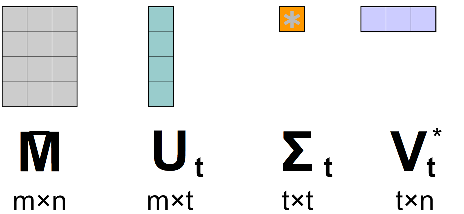
Based on the version of the SVD (full, compact, truncated, thin), the dimensions of the outputted matrices can vary (and it can make the SVD more or less applicable as you an encounter scalability issue)

Currently one of the most common of the version of SVD used is the truncated one and since the beginning of the 2000’s, the appearance of dedicated SVD for recommender system with for example [SVD++] that is designed to factorise matrice of implicit feedbacks.

Non-negative Matrix Factorization (NMF)

Origin: NMF is a technic that appeared in the 1990’s and developed originally by a Finnish group of researchers, but popularized by the investigation by Lee and Seung of Samsung in 1999.

Principle: The overall process is to decompose the original matrix in two sub matrices with the Feature matrix and the Coefficient matrix.

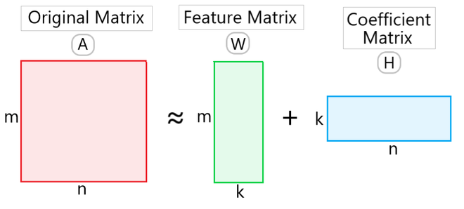
The process begins by initializing W and H with random non-negative values. Through an iterative process, these matrices are updated to minimize the difference between A and the product W×H. The updates are performed using multiplicative rules that ensure all elements remain non-negative.

Funk Matrix Factorization

Origin: Funk Matrix Factorization was popularized by Simon Funk during the Netflix Prize competition in 2006. It became widely known for its simplicity and effectiveness in improving the accuracy of recommendation systems.

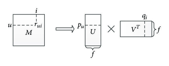
Principle: Funk Matrix Factorization decomposes the user-item interaction matrix into two lower-dimensional matrices, representing latent factors for users and items. The goal is to predict the missing entries in the original matrix by minimizing the prediction error of the known interactions. Funk MF leverages Stochastic Gradient Descent (SGD) to iteratively update the latent factor matrices, optimizing the approximation of the original matrix (it looks like and SVD but not really, so you can find it in the literature as funk SVD)

Probabilistic and Bayesian Matrix Factorization

Origin: Probabilistic Matrix Factorization (PMF) and its Bayesian variant (BMF) were introduced to address the uncertainty and sparsity issues in recommendation systems. PMF was popularized by Ruslan Salakhutdinov and Andriy Mnih in 2008.

Principle: Probabilistic Matrix Factorization models the user-item interaction matrix as a product of two lower-dimensional matrices. Each entry in the original matrix is treated as a Gaussian distribution, allowing for uncertainty in the predictions. The model aims to minimize the reconstruction error by adjusting the latent feature matrices through maximum likelihood estimation.

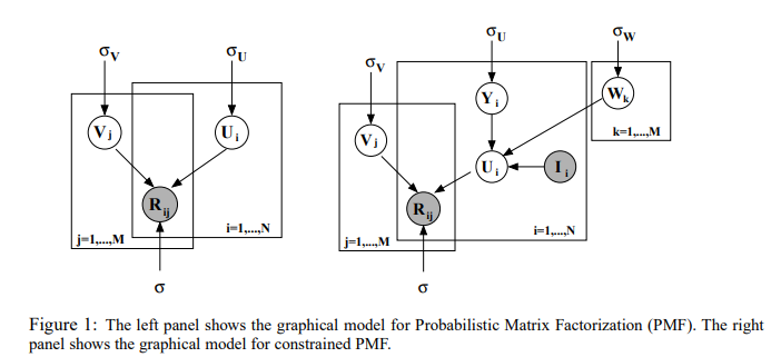
Bayesian Matrix Factorization extends PMF by incorporating prior distributions over the latent factors. This Bayesian approach provides a more flexible framework by capturing uncertainty in the model parameters. Using techniques like Markov Chain Monte Carlo (MCMC) or variational inference, BMF infers the posterior distributions of the latent factors, resulting in a more robust estimation especially when dealing with sparse data.

Alternating Least Squares (ALS)

Origin: The ALS algorithm is a popular approach for collaborative filtering in recommendation systems. It gained prominence in the early 2000s, notably used in the Netflix Prize competition to improve movie recommendations.

Principle: The ALS algorithm is used for matrix factorization, where the goal is to decompose a user-item interaction matrix into two lower-dimensional matrices: the user-feature matrix and the item-feature matrix. The key idea is to iteratively optimize one matrix while keeping the other fixed, alternating between the two until convergence.

It is particularly well-suited for distributed computing environments due to its independence of each user’s or item’s updates, enabling parallelization. This makes it a robust choice for large-scale recommendation systems.

Factorization Machines (FM)

Origin: Factorization Machines were introduced by Steffen Rendle in 2010 to handle sparse data and capture complex interactions between variables. They were developed to improve prediction accuracy in recommendation systems and other tasks involving high-dimensional data.

Principle: Factorization Machines combine the strengths of linear models with matrix factorization to model interactions between features. The key idea is to represent these interactions through factorized parameters, which allows the model to efficiently capture complex relationships in the data.

FMs can model all interactions between variables by representing them as the inner product of latent factor vectors, making them highly flexible. This approach enables FMs to learn interactions without explicitly defining them, allowing for scalable and accurate predictions even with sparse datasets.

Deep Learning-Based Matrix Factorization

Origin: Deep learning-based matrix factorization emerged as a natural extension of traditional matrix factorization techniques, incorporating neural networks to model complex interactions in data. This approach gained traction in the 2010s with the increased availability of computational resources and advances in neural network architectures, particularly for recommendation systems.

Principle: Deep learning-based matrix factorization enhances traditional matrix factorization by using neural networks to learn nonlinear relationships between users and items. Unlike classical approaches, which decompose a matrix into linear combinations of latent factors, deep learning methods use neural networks to capture more complex patterns.

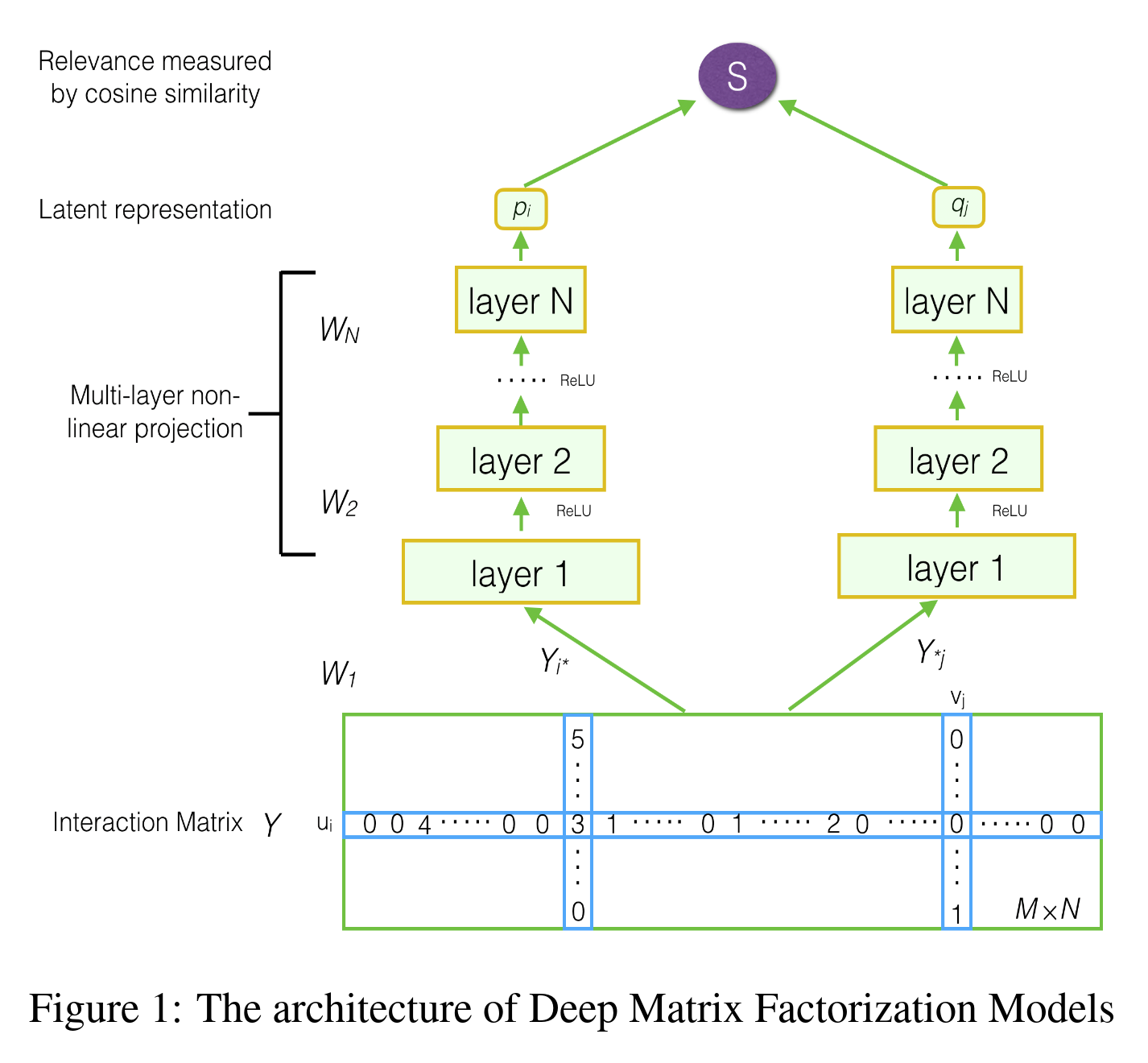
For example, the paper Neural Collaborative Filtering by Xiangnan He and colleagues from 2017 is very popular. They use a multi-layer perceptron (which replaces the dot product) to perform the factorization. Recent techniques like the variational autoencoder can also be used to reduce dimensions and build factors in a different, but very effective way. There’s a good illustration in this article with useful references.

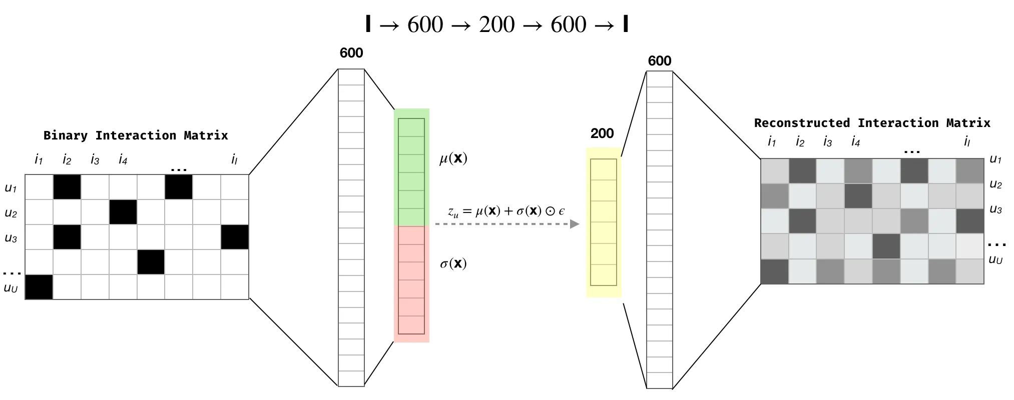
So, that was my general overview of matrix factorization for recommender systems. Now, let’s dive into a few considerations to keep in mind when working with these techniques.

Considerations around MF

Indexing the ratings

One of the most basic steps before applying any matrix factorization techniques is to index the user and item identifiers into the indices of the ratings matrix.

There are multiple ways to do this. In Python, you can easily use pandas functions for indexing. However, for something more scalable in a production environment (using Spark for example), I prefer to:

• Build mapping tables for users and items as they first appear in the application ecosystem. This process should be incremental to maintain efficiency.
• For associating indices, here’s a quick snippet of code in PySpark that I find useful:

Now that we have this mapping available, let’s dive deeper into where to start with matrix factorization.

Where to start ?

Here are my two recommendations for starting matrix factorization in the context of recommendations:

• For a local or single-machine setup, the Surprise package is definitely the place to start. This package is built on top of scikit-learn and implements multiple algorithms mentioned in previous sections (SVD, NMF, etc.).

Here’s a quick walkthrough:

• For a more distributed approach, PySpark MLlib has an implementation of the ALS algorithm that is very comprehensive. It allows you to set up modes to run with implicit feedback or enforce non-negative factors in the submatrices.

I believe these two packages provide a good starting point for anyone looking to use matrix factorization for recommendations.

Negative sampling as data augmentation

In various papers and implementations, the process of negative sampling is mentioned as a way to add new data to the training set. This operation is used in the context of implicit feedback, where the goal is to add some negative interactions. In scenarios with implicit feedback, you often only have positive feedback (such as clicks, or transactions), so negative sampling helps tackle the imbalance by adding a counterbalance, improving the learning of patterns in the ratings matrix.

There are different strategies to implement negative sampling:

• Pick random items to be labeled as negative.
• Pick items based on popularity (more popular items have a higher chance of being labeled negative since the user chose not to interact with them).

For me, this technic should be treated like a “hyperparameter” for the data behind the matrix factorization, a very powerful tool to use with the right precaution as you can inject biases in your data.

Evaluation

For this problem, evaluating the quality of the predicted ratings is crucial. Using RMSE or any other regression-related metric will do the job. Additionally, evaluating the ranking capabilities of the algorithm is interesting. A good approach for your test set is as follows:

• For each user in your test set, randomly pick X items (e.g., 100).
• Predict the rating for each selected user-item pair.
• Do the same for each item in the test set for that user.
• Evaluate classification metrics (like Hit Ratio or NDCG) by comparing the ranking of test set items with the randomly selected items. For positive ratings, you’d expect them to rank higher on the list.

This method is effective for evaluating the ranking ability of matrix factorization, but it requires a careful selection of items.

Scalability

This is a major consideration when you want to industrialize these kinds of algorithms. I have three rules to keep in mind.

First Rule: Don’t Build the Ratings Matrix! Or at least, don’t build it as a classical/dense matrix, because you would need to store a matrix with thousands of columns in memory. The better approach is to leverage the sparse matrix format, which can be offered by packages like Scipy or Cupy.

I benchmarked the memory size of a dense matrix (classical format) versus a sparse matrix with different configurations of users, items, and sparsity.

In configurations with high sparsity, the sparse matrix can be 6 to 7 times smaller in memory than the dense one so the sparse format is very efficient.

Second rule: Scale down users and items!

You don’t need to include all users. Users with low interaction levels can add noise, providing little value. Having a minimum ratings threshold for inclusion in the matrix is a good parameter to keep in mind (that will impact also the evaluation process). This approach is also discussed in some articles (1, 2) about recommender systems.

In some applications like Goodreads, users need a minimum number of interactions before recommendations are generated (not sure if they are using a matrix factorization under the hood)

As with users, it may not be necessary to include all items, especially those with low interactions (though these should be handled differently). In general, my suggestion is that you should potentially run Matrix Factorization on a subset of the item catalog. This subset should share something in common, like the same film category or a specific release period.

Playing with these elements of users and items, will impact your cold start strategies aka how to handle user or item with a lack of interactions because they are new or not so active, so be careful.

Don’t use it to make recommendations (directly)

This might sound odd, but let me explain:

• The range of predicted ratings may not match the real possible range of ratings. Factorization might not reduce the error sufficiently, and local minima could impact the rating mechanisms. It’s essential to build guardrails when using the predicted ratings.
• Some frameworks offer prebuilt methods on top of factorization, such as RecommendProductForUsers in PySpark. These functions work, but they may not handle specific conditions you might encounter when building recommendations (and not scaling well)

For example, when I use ALS, I prefer to build my own recommendation function with broadcasted item factors across the executors.

This setup works well when your item factors dataframe is not too large (thousand of items) , and it offers the flexibility to apply some custome rules like some weighting or filtering for specific items easily.

Let’s now conclude the article.

Closing notes

Ratings and Matrix Factorization are powerful tools for recommender systems. You can use them to compute user and item features that can be leveraged later to recommend content. These features can be easily integrated to build related entities functionalities in your application, like a “similar items” feature.

Regarding ratings and feedback, I strongly recommend using different types. If you have explicit ratings, use them as they are, but you should also build new implicit ratings to capture specific aspects of your application. For example, if you have click data on tiles in your application (in addition to explicit ratings), you should use this data as input for a new rating system that reflects user behavior related to clicks. You can combine different inputs to build these ratings, but avoid creating a single rating that tries to encompass everything. Consider that:

• New tracking data may emerge and alter your understanding of your application.
• It will become harder to explain the source of this rating, making it less useful for analysis and comprehension.

Different ratings (and the related factorized matrices) will help summarize a user’s preferences based on their interactions.

When it comes to choosing the right algorithm, it really depends on:

• The ratings used: The type and range of ratings will influence which algorithms you can use (like SVD vs. SVD++).
• The number of users and items: The scale of your data can impact algorithm selection.
• The sparsity of your dataset: The ratio of items to users affects the computing resources required and may influence your choice of algorithms.

I’ve noticed that algorithm selection is always a hot topic at recommender system conferences. For example, in this 2020 paper from Google, they benchmarked Neural Collaborative Filtering vs. MF , where the NCF exists since a few years now. Once again, it really depends on your use case, so you should benchmark them in your own environment before making a decision.

Finally, if you’re interested in learning more, here are some resources that might be useful:

• Matrix Factorization Techniques for Recommender Systems by Yehuda Koren, Robert Bell, and Chris Volinsky
• Recommenders, a GitHub repository managed by Microsoft that contains examples of MF
• TensorFlow Recommenders and TorchRec, which are also great sources of code around deep learning-based techniques
• Hagay Lupesko, a former director of Meta AI, made a recorded presentation for Open Data Science that is a great starting point on the topic of recommendation in general (with a dedicated section on deep learning based MF)

I hope you enjoy your reading. On my side, I will use this work as a starting point for future projects/articles that will focus more on:

• How to design a related item feature from scratch
• How to represent the factors for human (spoiler: there is, once again, dimensionality reduction involved)

So stay tuned 😉